This class represents a generalized linear model with Gamma distribution. It inherits from GLM and implements its functions that, for example, evaluate the conditional density and distribution functions.
Super classes
gofreg::ParamRegrModel -> gofreg::GLM -> GammaGLM
Methods
Method fit()
Calculates the maximum likelihood estimator for the model parameters based on given data.
Arguments
datatibble containing the data to fit the model to
params_initinitial value of the model parameters to use for the optimization (defaults to the fitted parameter values)
loglikfunction(data, model, params)defaults tologlik_xy()inplacelogical; ifTRUE, default model parameters are set accordingly and parameter estimator is not returned
Method f_yx()
Evaluates the conditional density function.
Arguments
tvalue(s) at which the conditional density shall be evaluated
xmatrix of covariates, each row representing one sample
paramsmodel parameters to use (
list()with tags beta and shape), defaults to the fitted parameter values
Method F_yx()
Evaluates the conditional distribution function.
Arguments
tvalue(s) at which the conditional distribution shall be evaluated
xmatrix of covariates, each row representing one sample
paramsmodel parameters to use (
list()with tags beta and shape), defaults to the fitted parameter values
Method F1_yx()
Evaluates the conditional quantile function.
Arguments
tvalue(s) at which the conditional quantile function shall be evaluated
xmatrix of covariates, each row representing one sample
paramsmodel parameters to use (
list()with tags beta and shape), defaults to the fitted parameter values
Method sample_yx()
Generates a new sample of response variables with the same conditional distribution.
Arguments
xmatrix of covariates, each row representing one sample
paramsmodel parameters to use (
list()with tags beta and shape), defaults to the fitted parameter values
Examples
# Use the built-in cars dataset
x <- datasets::cars$speed
y <- datasets::cars$dist
data <- dplyr::tibble(x=x, y=y)
# Create an instance of GammaGLM
model <- GammaGLM$new()
# Fit an Gamma GLM to the cars dataset
model$fit(data, params_init = list(beta=3, shape=1), inplace=TRUE)
params_opt <- model$get_params()
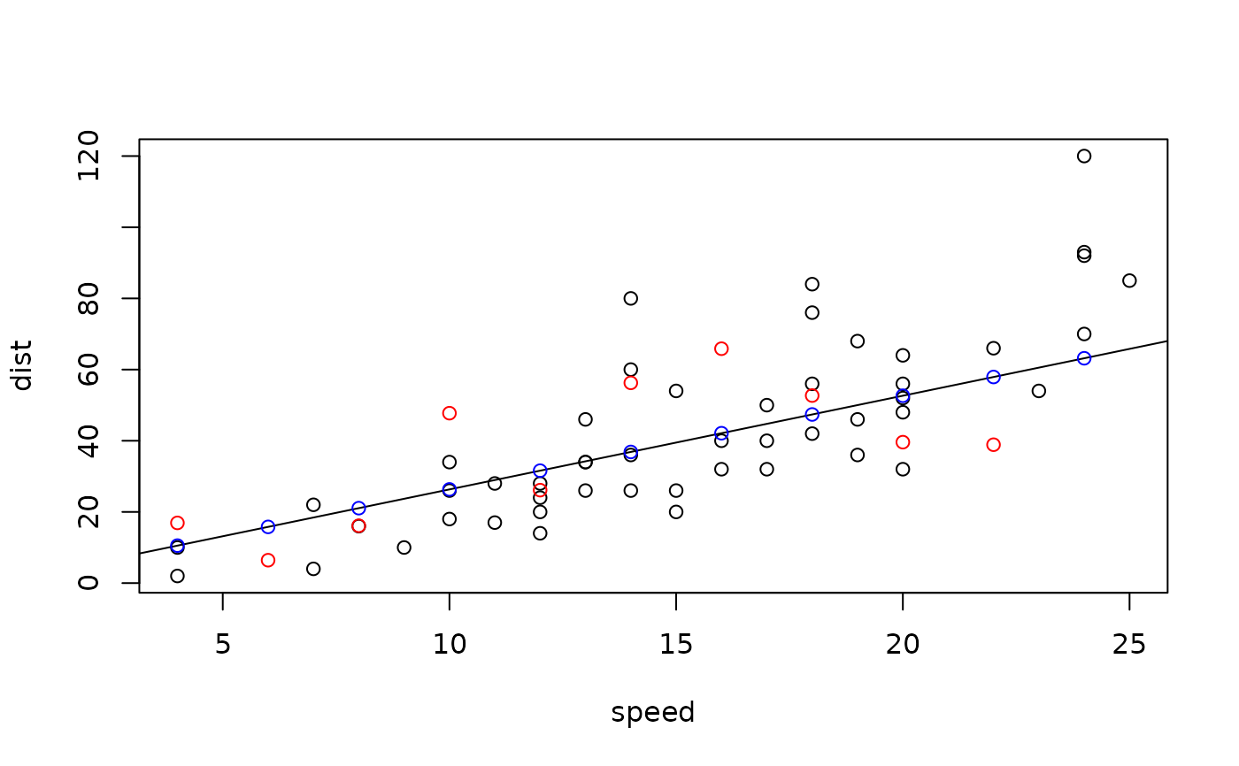
# Plot the resulting regression function
plot(datasets::cars)
abline(a = 0, b = params_opt$beta)
# Generate a sample for y for given x following the same distribution
x.new <- seq(min(x), max(x), by=2)
y.smpl <- model$sample_yx(x.new)
points(x.new, y.smpl, col="red")
# Evaluate the conditional density, distribution, quantile and regression
# function at given values
model$f_yx(y.smpl, x.new)
#> [1] 9.625437e-02 2.161378e-02 1.473827e-02 3.042118e-02 3.161315e-02
#> [6] 2.536134e-02 3.328638e-05 2.125175e-02 1.498809e-02 6.756113e-03
#> [11] 1.529278e-02
model$F_yx(y.smpl, x.new)
#> [1] 0.3873010 0.8855875 0.8976036 0.6536413 0.3119695 0.2335913 0.9996610
#> [8] 0.3332143 0.6616103 0.8655556 0.2639760
model$F1_yx(y.smpl, x.new)
#> Warning: NaNs produced
#> [1] NaN NaN NaN NaN NaN NaN NaN NaN NaN NaN NaN
y.pred <- model$mean_yx(x.new)
points(x.new, y.pred, col="blue")